In the last article, we discussed the importance of the dot product and how it appears everywhere in deep learning. We also saw briefly how the attention mechanism works.

Now I want to deep dive a little bit before we implement the architecture and look at the whole thing in detail.

Let's start with a simple example.

Suppose we have these two sentences:

Money bank river
River bank flows

Look at the word "bank."

The word is the same in both sentences, but the context around it is different.

In one case, we might be talking about a financial bank.

In the other, we are talking about the bank of a river.

A traditional word embedding gives the word "bank" a representation, but that representation is relatively fixed. It doesn't dynamically change depending on the sentence it appears in.

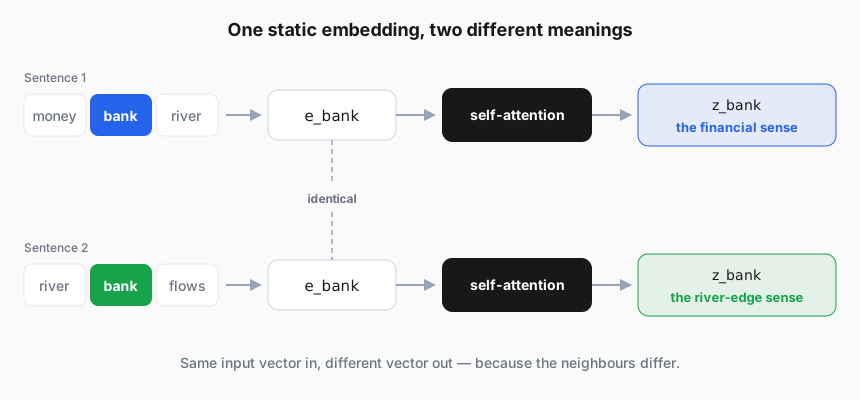
So intuitively, we need something more.

We want a representation that doesn't just contain information about the word itself, but can also incorporate information from the context surrounding that word.

And this is where self-attention becomes interesting.

---

Let's start with something very simple

Remember the nature of the dot product.

If two vectors point in similar directions, their dot product tends to be larger.

So let's say we have embeddings for:

$$e_{money}, e_{bank}, e_{river}$$

We can take the embedding of bank and compare it with every other embedding using the dot product:

$$e_{bank}\cdot e_{money}$$ $$e_{bank}\cdot e_{bank}$$ $$e_{bank}\cdot e_{river}$$

This gives us scalar scores telling us how strongly the bank embedding aligns with each of the other embeddings.

For example:

$$[0.2,\;1.0,\;0.7]$$

But these scores can be any real number. We want to convert them into weights that we can use to combine the information from the different words.

So we apply softmax:

$$softmax([0.2,1.0,0.7])$$

and get:

$$[0.21,\;0.46,\;0.34]$$

Now these numbers represent how much weight we're giving to each token.

And then we use these weights to take a weighted combination of the embeddings:

$$0.21e_{money} + 0.46e_{bank} + 0.34e_{river}$$

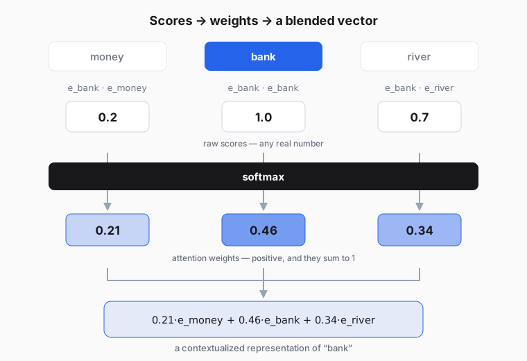
Now we have a new representation.

This representation contains information from the surrounding words.

We can call this a contextualized representation.

And intuitively, this is already starting to look like attention.

The whole thing in nine lines

That paragraph above is, quite literally, nine lines of code. Let's pick embeddings whose dot products with bank are exactly the numbers we just used:

import numpy as np

# Toy 2-D embeddings for "money bank river".
tokens = ["money", "bank", "river"]
E = np.array([
    [0.20, 0.98],   # money
    [1.00, 0.00],   # bank
    [0.70, 0.71],   # river
])

def softmax(x):
    e = np.exp(x - x.max())
    return e / e.sum()

e_bank = E[1]

scores  = E @ e_bank        # dot product of "bank" with every token
weights = softmax(scores)   # turn scores into weights that sum to 1
z_bank  = weights @ E       # blend the embeddings using those weights

print("scores  ", np.round(scores, 2))
print("weights ", np.round(weights, 2))
print("z_bank  ", np.round(z_bank, 3))

Running it:

scores   [0.2 1.  0.7]
weights  [0.21 0.46 0.34]
z_bank   [0.734 0.441]

z_bank is no longer the row we started with. It has drifted away from [1.0, 0.0] and picked up a bit of money and a bit of river along the way.

That drift is the context.

---

But there is a problem

Let's stop here and ask ourselves an important question.

We're trying to build a neural network that can learn from data and eventually predict the next token.

But what have we actually learned here?

Nothing.

Look at the code again. There is no variable in it that training could ever change. E comes from the embedding table, and everything after that — the dot product, the softmax, the weighted sum — is a fixed formula.

We're simply taking the embeddings, calculating their similarity using a dot product, applying softmax and taking a weighted average.

There are no learnable parameters in this process that tell the model what kind of relationships it should learn.

We're basically applying the same fixed operation to whatever sentence we give it.

And there's a subtler problem hiding in there too. We used the same vector for two different jobs: e_bank was both the thing doing the asking and one of the things being asked. A word's "what am I looking for?" and its "what do I have to offer?" are not the same question, but this formulation forces them to share one vector.

And this is where we introduce something important:

learnable weight matrices.

Instead of directly using the original embedding for everything, we transform our embeddings into three different representations:

$$\boxed{Q=XW_Q}$$ $$\boxed{K=XW_K}$$ $$\boxed{V=XW_V}$$

where $W_Q$, $W_K$, and $W_V$ are learnable parameters.

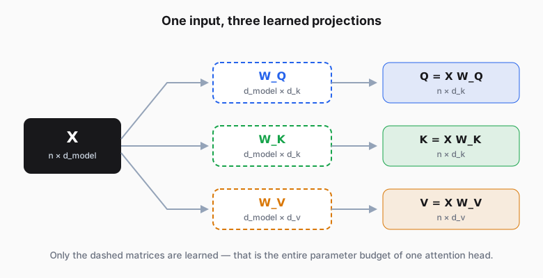
Now the model can actually learn from data how it should construct these representations.

And this gives us the famous:

$$\boxed{ Attention(Q,K,V) = softmax\left( \frac{QK^T}{\sqrt{d_k}} \right)V }$$

---

So what are Q, K and V actually doing?

Let's go back to our intuition.

Suppose we have:

The cat drank the milk because it was thirsty.

Look at the word "it."

The model needs to understand what "it" is referring to.

We can think of the Query of "it" as asking:

"What am I looking for?"

The other tokens have Keys.

So we calculate:

$$Q_{it}K_{cat}^T$$ $$Q_{it}K_{drank}^T$$ $$Q_{it}K_{milk}^T$$ $$Q_{it}K_{thirsty}^T$$

These give us scores representing how strongly the query aligns with each key.

But notice something: "it" is not special. Every token forms a query and looks at every token's key, all at once. So what we actually get is not a single row of scores — it's a full $n \times n$ grid, one row per token:

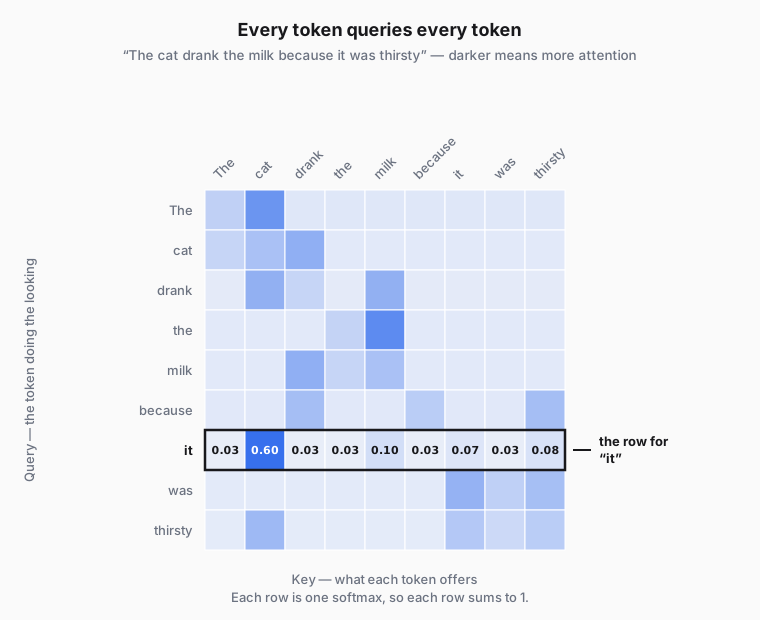
That grid is why it's called self-attention: the sentence is attending to itself.

Read along the highlighted row and you can see the model resolving the pronoun — "it" puts about 0.60 of its weight on cat, and spreads the rest thinly over everything else.

The exact numbers aren't important here.

The important idea is:

QKᵀ tells us where to look.

But we still need the actual information from those tokens.

And this is where V comes in.

The Key is used for matching.

The Value contains the information we actually retrieve.

So once we have the attention weights, we multiply them by the Values:

$$\text{Attention Weights}\times V$$

and get the attended representation.

So you can think about the whole process like this:

Q: What am I looking for?
K: What do I contain that might match your question?
V: If you choose me, what information should I give you?

This is the intuition behind Query, Key and Value.

---

Putting everything together

Here is the whole thing in one picture, with the shapes written in — because once you can track the shapes, the equation stops being intimidating:

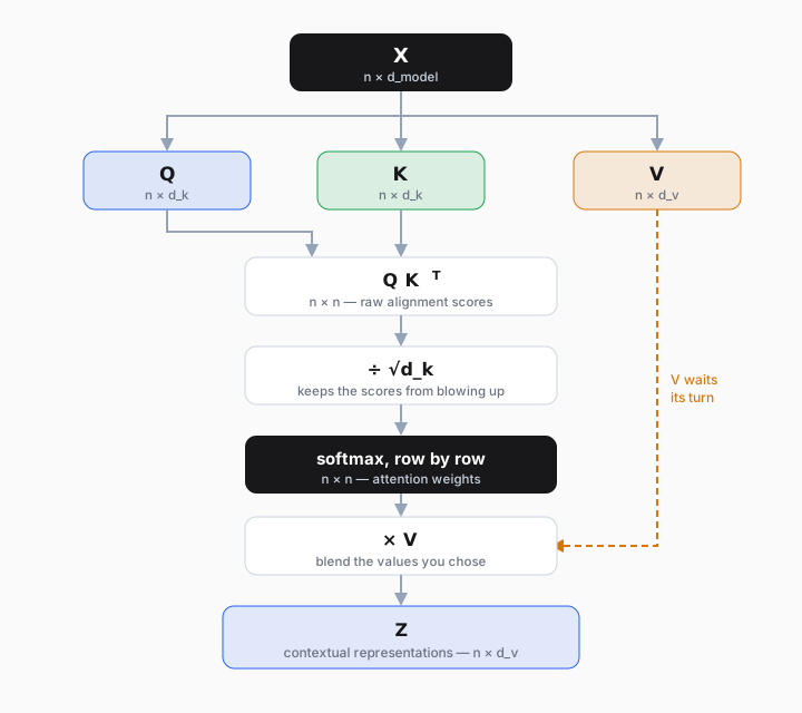
Two details worth pausing on.

The scaling by $\sqrt{d_k}$. $Q$ and $K$ have $d_k$ dimensions, so their dot product is a sum of $d_k$ terms. As $d_k$ grows, those sums drift further from zero. Feed very large numbers into softmax and it saturates — one weight goes to ~1, the rest go to ~0, and the gradients flatten out. Dividing by $\sqrt{d_k}$ keeps the scores in a range where softmax still has something to say.

The softmax is row-wise. Each row is one token's question, so each row gets its own softmax and each row sums to 1. It is not one softmax over the whole matrix.

And now the code. This is the same nine-line idea as before, with the three projections added:

import numpy as np

rng = np.random.default_rng(0)

tokens = ["the", "cat", "drank", "the", "milk"]
n, d_model, d_k, d_v = len(tokens), 8, 4, 4

X = rng.normal(size=(n, d_model))          # token embeddings

W_Q = rng.normal(size=(d_model, d_k)) * 0.5
W_K = rng.normal(size=(d_model, d_k)) * 0.5
W_V = rng.normal(size=(d_model, d_v)) * 0.5

def softmax(x, axis=-1):
    e = np.exp(x - x.max(axis=axis, keepdims=True))
    return e / e.sum(axis=axis, keepdims=True)

def self_attention(X, W_Q, W_K, W_V):
    Q = X @ W_Q                              # (n, d_k)
    K = X @ W_K                              # (n, d_k)
    V = X @ W_V                              # (n, d_v)

    scores  = Q @ K.T / np.sqrt(K.shape[-1]) # (n, n)
    weights = softmax(scores, axis=-1)       # (n, n), each row sums to 1
    return weights @ V, weights              # (n, d_v), (n, n)

Z, A = self_attention(X, W_Q, W_K, W_V)

print("X shape", X.shape, "-> Z shape", Z.shape)
print("\nattention weights (rows = queries, cols = keys)")
print("            " + "".join(f"{t:>8}" for t in tokens))
for tok, row in zip(tokens, A):
    print(f"{tok:>10}  " + "".join(f"{w:8.2f}" for w in row))
print("\nrow sums", np.round(A.sum(axis=1), 6))

Output:

X shape (5, 8) -> Z shape (5, 4)

attention weights (rows = queries, cols = keys)
                 the     cat   drank     the    milk
       the      0.03    0.32    0.12    0.51    0.02
       cat      0.56    0.13    0.05    0.02    0.24
     drank      0.45    0.31    0.02    0.08    0.14
       the      0.08    0.15    0.50    0.16    0.11
      milk      0.02    0.38    0.20    0.39    0.02

row sums [1. 1. 1. 1. 1.]

Those five lines inside self_attention are the entire mechanism. Everything else in a transformer block is scaffolding around them.

But look closely at that matrix, because there's an easy trap here. drank is paying 0.45 of its attention to the first the, and cat is doing much the same. This grid means nothing. $W_Q$, $W_K$ and $W_V$ came out of a random number generator, so the pattern is noise.

The mechanism is what the code gives you. The meaning only shows up after those three matrices have been trained — the pronoun-resolving grid from earlier is what a trained head can look like, not what an untrained one does.

---

In the next article, I want to talk about one important limitation in the simple intuition we developed above, and how the actual Transformer architecture addresses it.