Attention: Causal Masking, MHA, MQA and GQA

At the end of the last article I said there was one important limitation in the intuition we built.

Here it is.

We computed attention over the whole matrix. Every token formed a query, and that query was compared against every key in the sentence. Including the keys of tokens that come after it.

Go back and look at that attention grid again. The row for "it" was reading was and thirsty, two words that sit to its right.

For a model whose entire job is to predict the next token, that is a problem.

Why looking ahead breaks training

Let's be precise about why, because the usual hand-wave is that "the model shouldn't know the future" and that is not quite the reason.

Here is the reason.

During training we do not feed the model one token at a time. We hand it the whole sequence at once and ask it to predict the next token at every position simultaneously. Position 1 predicts token 2, position 2 predicts token 3, and so on down the sequence. That is what makes training a transformer fast.

Now suppose position 2 is allowed to attend to position 3.

Position 2 is being asked to predict token 3. And attention just handed it token 3.

The model does not learn anything. It learns to copy. The loss goes to nearly zero on the training set and the model is useless the moment you ask it to generate something it has not already been given.

This is label leakage, and it is a training bug, not a philosophical one.

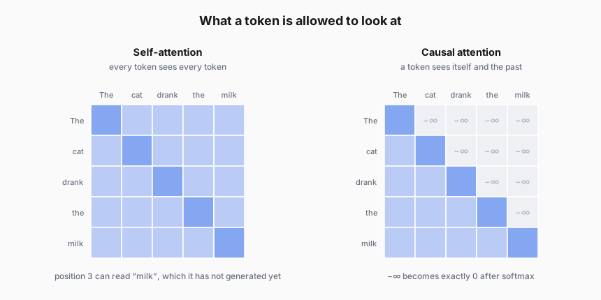
Causal attention

The fix is simple, and it happens in exactly one place.

Before the softmax, we take every score that points forward in time and set it to $-\infty$.

Why $-\infty$ and not zero?

Because zero is a perfectly respectable score. $e^0 = 1$, so a zero score still gets a share of the attention weight after softmax. Setting a score to zero does not remove a token, it just makes it averagely interesting.

What we want is a weight of exactly zero coming out of the softmax. So we need the input to be the value that softmax maps to zero:

$$\lim_{x \to -\infty} \frac{e^{x}}{\sum e^{x_j}} = 0$$

In floating point, exp(-inf) really does evaluate to 0.0, so the masked positions contribute nothing to the sum and nothing to the weighted average of the values.

The mask is applied to the scores, not to the weights. If you mask after the softmax you have to renormalize by hand, and you will get it wrong eventually.

import numpy as np

def softmax(x, axis=-1):
    e = np.exp(x - x.max(axis=axis, keepdims=True))
    return e / e.sum(axis=axis, keepdims=True)

def causal_attention(Q, K, V):
    n, d_k = Q.shape

    scores = Q @ K.T / np.sqrt(d_k)                  # (n, n)

    # True everywhere we are not allowed to look:
    # strictly above the diagonal, so column > row.
    future = np.triu(np.ones((n, n), dtype=bool), k=1)
    scores = np.where(future, -np.inf, scores)

    weights = softmax(scores, axis=-1)               # row t is 0 past column t
    return weights @ V, weights

Row 0 attends only to itself. Row 1 attends to positions 0 and 1. The last row is the only one that sees the whole sentence, and that is exactly right, because the last row is the only position with nothing left to predict.

One detail worth noticing: every row still sums to 1. Masking does not shrink the attention, it redistributes it over a smaller set of tokens.

Two different questions

Before going further it is worth separating two things that are easy to blur together, because the rest of this article is about the second one.

What is a token allowed to look at? That is masking. Causal, bidirectional, sliding window, and so on.

How many different ways can it look? That is heads. MHA, MQA, GQA.

These are independent. A model can be causal and multi-head, causal and single-head, bidirectional and grouped. Changing one does not change the other. BERT is bidirectional multi-head. GPT is causal multi-head.

Mixing these two up is the most common confusion in this area, so it is worth holding them apart deliberately.

Multi-head attention

So far one query vector produced one set of attention weights, which produced one weighted average.

That is a single opinion about the sentence.

Think about what a word actually relates to. Take "drank" in our sentence. It has a subject, cat. It has an object, milk. It has a tense. It has a position. Those are four different kinds of relationship, and we are asking a single softmax distribution to encode all of them at once.

It cannot. A probability distribution that has to put weight on cat and on milk for different reasons ends up putting mediocre weight on both, and the two signals get averaged into mush.

So we run attention several times in parallel and let each copy specialize.

The part people get wrong is the cost. Multi-head attention is not $h$ times more expensive than single-head attention, because we do not duplicate the model dimension. We split it.

$$head\_dim = \frac{d_{model}}{h}$$

With $d_{model} = 512$ and $h = 8$, each head works in 64 dimensions, not 512. Eight heads of 64 is the same total width as one head of 512. The FLOPs are roughly unchanged. You get eight perspectives for approximately the price of one.

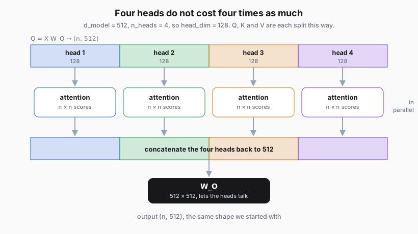
After the heads run, we lay their outputs back side by side to get a $(n, d_{model})$ matrix again, and pass it through one more learned matrix $W_O$. That last projection matters more than it looks. Without it the heads would be eight independent strips that never mix. $W_O$ is what lets information found by head 3 reach the part of the vector that head 7 wrote.

def multi_head_attention(X, W_Q, W_K, W_V, W_O, n_heads, causal=True):
    """
    X    : (n, d_model)
    W_Q  : (d_model, d_model)   same for W_K, W_V, W_O
    """
    n, d_model = X.shape
    head_dim = d_model // n_heads

    # Project once, then split the last axis into heads.
    # (n, d_model) -> (n, n_heads, head_dim) -> (n_heads, n, head_dim)
    Q = (X @ W_Q).reshape(n, n_heads, head_dim).transpose(1, 0, 2)
    K = (X @ W_K).reshape(n, n_heads, head_dim).transpose(1, 0, 2)
    V = (X @ W_V).reshape(n, n_heads, head_dim).transpose(1, 0, 2)

    # Batched over heads: (h, n, head_dim) @ (h, head_dim, n) -> (h, n, n)
    scores = Q @ K.transpose(0, 2, 1) / np.sqrt(head_dim)

    if causal:
        future = np.triu(np.ones((n, n), dtype=bool), k=1)
        scores = np.where(future, -np.inf, scores)   # broadcasts over heads

    heads = softmax(scores, axis=-1) @ V             # (h, n, head_dim)

    # Put the heads back side by side, then let them mix.
    concat = heads.transpose(1, 0, 2).reshape(n, d_model)   # (n, d_model)
    return concat @ W_O                                     # (n, d_model)

The two transpose calls are the only fiddly part. The first moves n_heads in front of the sequence axis so the matmul batches over heads. The second undoes it so the reshape puts each token's heads next to each other rather than interleaving tokens.

Getting that second transpose wrong is a real bug and a quiet one. The shapes still work out, the model still trains, it just trains worse than it should.

The problem nobody sees until they deploy

Multi-head attention is what everyone reaches for. So why do modern models not use it?

The answer is not training. It is generation.

When a model generates text, it produces one token at a time, and each new token has to attend to every token before it. Recomputing the keys and values for the whole prefix on every single step would be quadratic work for no reason, since those keys and values never change once computed.

So we cache them. That cache is the KV cache, and it grows with every token generated.

Its size is:

$$2 \times layers \times kv\_heads \times head\_dim \times bytes \times sequence\_length$$

The 2 is for K and V. Notice what is not in that formula: the batch is on the outside, so every concurrent request pays this in full.

Put real numbers in it.

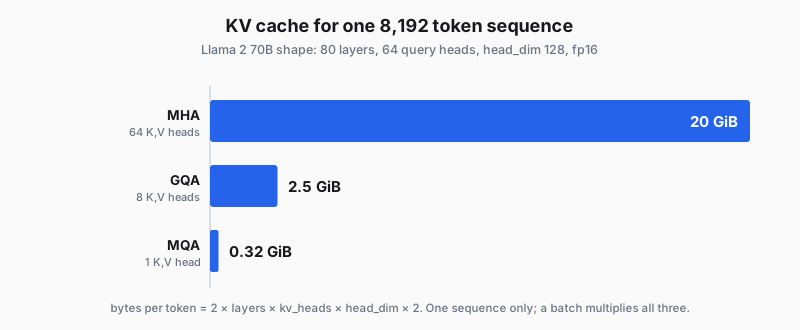
Twenty gigabytes. For one conversation, on a model whose weights are already using most of the GPU.

And memory is only half of it. Generating a single token requires reading that entire cache out of HBM. Autoregressive decoding is not compute bound, it is memory bandwidth bound. The GPU spends most of its time waiting for the KV cache to arrive, not multiplying anything.

Which means shrinking the cache does not just let you fit longer contexts. It directly makes generation faster.

Look at the formula again and ask which term you can actually reduce.

layers and head_dim are the model's architecture. sequence_length is the user's. bytes is quantization, a different lever.

That leaves kv_heads.

MQA: one key and value for everybody

The most aggressive answer, and the first one historically, is Multi-Query Attention.

Keep all $h$ query heads. Project one key head and one value head, and let every query head attend against that same pair.

The KV cache shrinks by a factor of $h$. In the chart above, 20 GiB becomes 0.32 GiB.

The cost is representational. The whole argument for multiple heads was that different heads should look for different things, and a query head can only look for what the shared keys make findable. You keep $h$ different questions but you collapse the index they are searching against down to one.

In practice MQA does lose quality, and it can be unstable to train. That is the honest tradeoff, and it is why MQA is not the default.

GQA: the dial in between

Grouped-Query Attention is the observation that MHA and MQA are the two ends of one axis, and nothing forces you to sit at either end.

Split the $h$ query heads into $g$ groups. Give each group its own key and value head. Every query head in a group shares that pair.

$g = h$ gives you MHA. $g = 1$ gives you MQA. Anything in between is GQA.

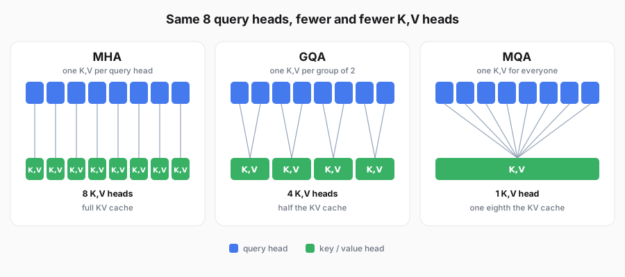
The empirical result is the interesting part: quality does not degrade linearly as you cut key and value heads. Most of the loss happens on the last step down to a single head. Going from 64 KV heads to 8 costs very little, while already recovering 87% of the memory. That is why 8 is such a common choice, and why GQA is now the default in most open-weight models rather than a compromise anyone apologizes for.

Here is the whole family as one function. The only new idea is np.repeat.

def grouped_query_attention(X, W_Q, W_K, W_V, W_O,
                            n_heads, n_kv_heads, causal=True):
    """
    W_Q : (d_model, n_heads    * head_dim)
    W_K : (d_model, n_kv_heads * head_dim)   <- this is the saving
    W_V : (d_model, n_kv_heads * head_dim)

    n_kv_heads == n_heads -> MHA
    n_kv_heads == 1       -> MQA
    anything between      -> GQA
    """
    n, d_model = X.shape
    head_dim = d_model // n_heads
    group_size = n_heads // n_kv_heads      # query heads per K,V head

    # Queries keep every head.
    Q = (X @ W_Q).reshape(n, n_heads, head_dim).transpose(1, 0, 2)

    # Keys and values get far fewer. This is the entire trick.
    K = (X @ W_K).reshape(n, n_kv_heads, head_dim).transpose(1, 0, 2)
    V = (X @ W_V).reshape(n, n_kv_heads, head_dim).transpose(1, 0, 2)

    # Hand each K,V head to the query heads in its group.
    # repeat gives [kv0, kv0, kv1, kv1, ...], which is the grouping we want.
    # tile would give [kv0, kv1, kv0, kv1, ...], which is not.
    K = np.repeat(K, group_size, axis=0)    # (n_heads, n, head_dim)
    V = np.repeat(V, group_size, axis=0)    # (n_heads, n, head_dim)

    scores = Q @ K.transpose(0, 2, 1) / np.sqrt(head_dim)

    if causal:
        future = np.triu(np.ones((n, n), dtype=bool), k=1)
        scores = np.where(future, -np.inf, scores)

    heads = softmax(scores, axis=-1) @ V
    concat = heads.transpose(1, 0, 2).reshape(n, d_model)
    return concat @ W_O

One thing this code makes clear that a diagram cannot: the repeat is a lie we tell for readability. A real implementation never materializes those copies, because materializing them would undo the entire point. The kernel indexes into the small K and V directly. Written out like this the arithmetic is identical and the memory saving is zero, so treat this version as a specification rather than something to ship.

Where this leaves us

	K,V heads	KV cache	What you give up
MHA	$h$	full	nothing
GQA	$g$	$h/g$ smaller	very little, if $g$ is not tiny
MQA	1	$h$ smaller	real quality, sometimes stability

The thing to carry away is that none of these change what attention is. The equation from the last article is untouched. What changes is how many independent key and value projections you are willing to store, and that decision is made almost entirely by inference economics rather than by modeling taste.

Which is a pattern worth noticing. A surprising amount of modern architecture is not "what represents language best" but "what fits in memory while a thousand users are talking to it at once."

There is a fourth answer to this same question that goes further than GQA. Instead of sharing key and value heads, Multi-head Latent Attention compresses K and V into a low rank latent vector and caches that instead, decompressing on the fly. It is what DeepSeek uses, it interacts awkwardly with rotary position embeddings, and it deserves its own article rather than a paragraph at the end of this one.

That is where we go next.