I Trained a GPT-2 From Scratch on Tiny Shakespeare

For a while I have been writing about attention from the inside: the dot product, self-attention, causal masking and MHA / GQA, then MLA.

At some point reading about transformers stops being enough.

You want to put the pieces together, hit train, watch the loss fall, and then ask the model to finish a line that starts with ROMEO:.

So I did that.

A self-contained notebook. GPT-2 style architecture. Tiny Shakespeare. GPT-2 BPE via tiktoken. One Tesla T4 on Colab.

This is not a research run. It is the run you do when you want the stack to stop feeling abstract.

Below is the path I took, with the code that actually mattered and what each piece is doing.

What I was actually trying to learn

Not "can I beat OpenAI."

I wanted answers to smaller questions:

• Can I wire token embeddings, positional embeddings, causal multi-head attention, MLP blocks, and an LM head without importing someone else's model zoo?
• Does the training loop I think I understand (warmup, AdamW, grad clip, gradient accumulation) behave the way the blog posts say it does?
• After a short run on a tiny corpus, does the model sound even a little bit like Shakespeare?

If those three work, the architecture articles stop being vibes and start being a system you can touch.

The honest config

The notebook title says GPT-2 Small (~124M). That is the shape people mean when they say GPT-2 Small: d_model=768, 12 layers, 12 heads, context 1024, vocab 50,257.

On a free T4, that is painful.

So I ran a smaller cousin of the same architecture:

@dataclass
class GPTConfig:
    vocab_size: int = 50257   # GPT-2 BPE
    d_model: int = 384
    num_layers: int = 6
    num_heads: int = 6
    block_size: int = 256     # drop further if OOM
    dropout: float = 0.1
    bias: bool = True         # GPT-2 uses bias in Linears / LayerNorm


BATCH_SIZE = 4
GRAD_ACCUM_STEPS = 8          # effective batch = 4 * 8 = 32
MAX_ITERS = 1000
LEARNING_RATE = 3e-4
WEIGHT_DECAY = 0.1
GRAD_CLIP = 1.0
WARMUP_ITERS = 100

Knob	What I used
d_model	384
layers	6
heads	6
block_size	256
vocab	50,257 (GPT-2 BPE)
parameters	~30M
device	Tesla T4

Same ideas. Same components. Just fewer of them so training finishes in minutes instead of hours.

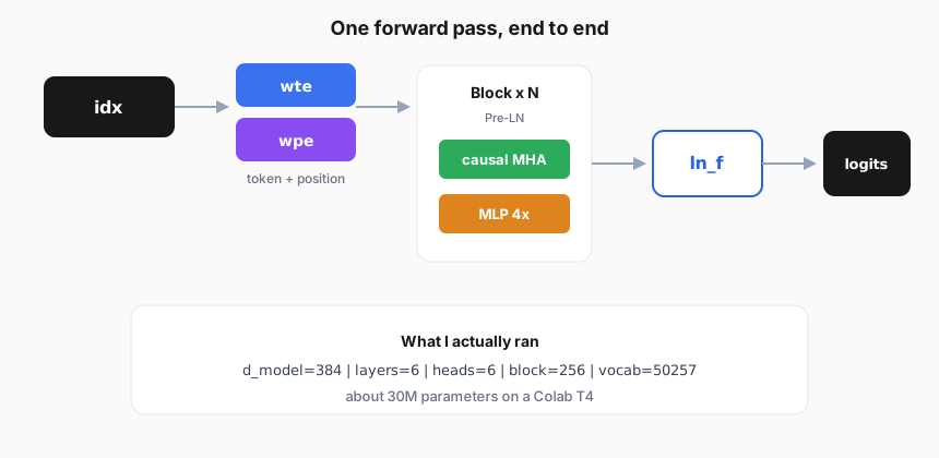
This is an important habit: keep the architecture recognizable, shrink the widths until the experiment fits the GPU you have.

Data: Tiny Shakespeare + real BPE

Tiny Shakespeare is about 1.1M characters. I still used GPT-2 BPE, not character-level tokenization.

Why?

Because I wanted the embedding matrix to look like the real GPT-2 setup. Char-level Tiny Shakespeare has a tiny alphabet. That hides how much of GPT-2's parameter count lives in the vocabulary path.

import tiktoken

text = DATA_PATH.read_text(encoding="utf-8")

enc = tiktoken.get_encoding("gpt2")
assert enc.n_vocab == config.vocab_size

token_ids = torch.tensor(enc.encode_ordinary(text), dtype=torch.long)
n = int(0.9 * len(token_ids))
train_ids = token_ids[:n]
val_ids = token_ids[n:]
# tokens: 338,025 | train=304,222 | val=33,803

encode_ordinary is the important call here. It turns raw text into the same integer stream GPT-2 was designed around.

Turning a token stream into training pairs

The training objective is next-token prediction. Take a window of tokens x. Shift it by one to get targets y. Predict every position in one forward pass.

def get_batch(split: str):
    data = train_ids if split == "train" else val_ids
    ix = torch.randint(len(data) - config.block_size, (BATCH_SIZE,))
    x = torch.stack([data[i : i + config.block_size] for i in ix])
    y = torch.stack([data[i + 1 : i + 1 + config.block_size] for i in ix])
    return x.to(device), y.to(device)

That is the entire dataset logic for a nanoGPT-style loop.

• x[t] is the context the model is allowed to see
• y[t] is the token it should predict at that position
• random starts keep the batches cheap and mixed

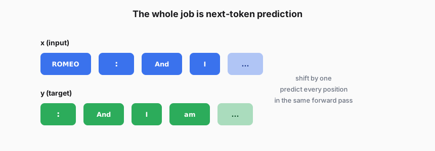
If you have been following the attention series, this is where causal masking stops being a diagram and becomes the only thing stopping the model from cheating. Without the mask, position t could attend to y[t] through the future tokens and the loss would become a copy exercise.

The model, in the order I built it

I inlined everything in the notebook. No from models import GPT.

Causal multi-head attention

This is the piece the earlier articles were building toward.

One linear layer produces Q, K, and V together. Split into heads. Scale. Mask the future with -inf. Softmax. Mix values. Project back.

class CausalSelfAttention(nn.Module):
    def __init__(self, cfg: GPTConfig):
        super().__init__()
        assert cfg.d_model % cfg.num_heads == 0
        self.num_heads = cfg.num_heads
        self.head_size = cfg.d_model // cfg.num_heads
        self.d_model = cfg.d_model

        self.c_attn = nn.Linear(cfg.d_model, 3 * cfg.d_model, bias=cfg.bias)
        self.c_proj = nn.Linear(cfg.d_model, cfg.d_model, bias=cfg.bias)
        self.attn_dropout = nn.Dropout(cfg.dropout)
        self.resid_dropout = nn.Dropout(cfg.dropout)

        # lower-triangular causal mask, stored once
        self.register_buffer(
            "mask",
            torch.tril(torch.ones(cfg.block_size, cfg.block_size)).view(
                1, 1, cfg.block_size, cfg.block_size
            ),
        )

    def forward(self, x):
        B, T, C = x.shape

        qkv = self.c_attn(x)                          # [B, T, 3C]
        q, k, v = qkv.split(self.d_model, dim=2)

        # [B, nh, T, hs]
        q = q.view(B, T, self.num_heads, self.head_size).transpose(1, 2)
        k = k.view(B, T, self.num_heads, self.head_size).transpose(1, 2)
        v = v.view(B, T, self.num_heads, self.head_size).transpose(1, 2)

        att = (q @ k.transpose(-2, -1)) * (1.0 / math.sqrt(self.head_size))
        att = att.masked_fill(self.mask[:, :, :T, :T] == 0, float("-inf"))
        att = F.softmax(att, dim=-1)
        att = self.attn_dropout(att)

        y = att @ v                                   # [B, nh, T, hs]
        y = y.transpose(1, 2).contiguous().view(B, T, C)
        return self.resid_dropout(self.c_proj(y))

A few lines worth pausing on:

• c_attn projects to 3 * d_model once, then we split. That is cheaper and cleaner than three separate modules.
• The transpose(1, 2) puts heads in front so the matmul batches over heads.
• masked_fill(..., -inf) is the causal rule from the previous article, now living inside real training.
• c_proj is the output mix. Without it, the heads stay as separate strips that never talk to each other.

MLP

After attention mixes information across tokens, the MLP processes each token independently.

class MLP(nn.Module):
    def __init__(self, cfg: GPTConfig):
        super().__init__()
        self.fc = nn.Linear(cfg.d_model, 4 * cfg.d_model, bias=cfg.bias)
        self.proj = nn.Linear(4 * cfg.d_model, cfg.d_model, bias=cfg.bias)
        self.dropout = nn.Dropout(cfg.dropout)

    def forward(self, x):
        x = self.fc(x)
        x = F.gelu(x)      # GPT-2 style
        x = self.proj(x)
        return self.dropout(x)

Expand to 4 * d_model, nonlinearity, project back. That expansion is where a lot of the model's capacity sits. Attention decides who to listen to. The MLP decides what to do with what it heard.

Transformer block (Pre-LN)

GPT-2 uses residual blocks with LayerNorm before each sublayer:

class Block(nn.Module):
    def __init__(self, cfg: GPTConfig):
        super().__init__()
        self.ln1 = nn.LayerNorm(cfg.d_model)
        self.attn = CausalSelfAttention(cfg)
        self.ln2 = nn.LayerNorm(cfg.d_model)
        self.mlp = MLP(cfg)

    def forward(self, x):
        x = x + self.attn(self.ln1(x))
        x = x + self.mlp(self.ln2(x))
        return x

This is short on purpose.

The residual x + ... is what lets gradients travel through a deep stack. Pre-LN (ln before the sublayer) is the modern default because it trains more stably than the original Post-LN layout.

Full GPT-2 wrapper

Now glue it together:

class GPT2(nn.Module):
    def __init__(self, cfg: GPTConfig):
        super().__init__()
        self.config = cfg

        self.wte = nn.Embedding(cfg.vocab_size, cfg.d_model)     # token
        self.wpe = nn.Embedding(cfg.block_size, cfg.d_model)     # learned positions
        self.drop = nn.Dropout(cfg.dropout)
        self.blocks = nn.ModuleList([Block(cfg) for _ in range(cfg.num_layers)])
        self.ln_f = nn.LayerNorm(cfg.d_model)
        self.lm_head = nn.Linear(cfg.d_model, cfg.vocab_size, bias=False)

        # weight tying: lm_head shares wte
        self.lm_head.weight = self.wte.weight

        self.apply(self._init_weights)
        for pn, p in self.named_parameters():
            if pn.endswith("c_proj.weight") or pn.endswith("proj.weight"):
                torch.nn.init.normal_(p, mean=0.0, std=0.02 / math.sqrt(2 * cfg.num_layers))

    def forward(self, idx, targets=None):
        B, T = idx.shape
        pos = torch.arange(0, T, dtype=torch.long, device=idx.device)
        x = self.drop(self.wte(idx) + self.wpe(pos))

        for block in self.blocks:
            x = block(x)
        x = self.ln_f(x)
        logits = self.lm_head(x)                      # [B, T, vocab]

        loss = None
        if targets is not None:
            loss = F.cross_entropy(
                logits.view(-1, logits.size(-1)),
                targets.view(-1),
            )
        return logits, loss

What this is saying in plain language:

1. Look up token vectors and position vectors, add them.
2. Run N residual blocks.
3. Final LayerNorm.
4. Project to vocab logits.
5. If we have targets, flatten and run cross-entropy over every position.

Weight tying is the detail people often skip. The matrix that turns token ids into vectors is also the matrix that turns hidden states back into vocab logits. Same space, shared parameters. That is why the embedding table dominates the parameter count when the vocab is 50k.

On my run this printed:

parameters: 30.04M  (non-embedding ≈ 10.65M)
config: d_model=384 layers=6 heads=6 block=256

Most of the 30M is the embedding / LM-head path. The "thinking" trunk is closer to 11M.

Training setup

This is the part people skip when they only copy architecture diagrams.

Optimizer and schedule

AdamW with decay on 2D weights, no decay on biases / LayerNorm / embeddings. Linear warmup, then cosine decay:

def get_lr(it):
    if it < WARMUP_ITERS:
        return LEARNING_RATE * (it + 1) / WARMUP_ITERS
    decay_ratio = (it - WARMUP_ITERS) / max(1, MAX_ITERS - WARMUP_ITERS)
    coeff = 0.5 * (1.0 + math.cos(math.pi * decay_ratio))
    return LEARNING_RATE * 0.1 + coeff * (LEARNING_RATE - LEARNING_RATE * 0.1)

Warmup stops the first steps from swinging too hard. Cosine decay eases the model into a quieter end of training.

The training loop

The loop itself is short. The important idea is gradient accumulation.

for it in range(MAX_ITERS):
    lr = get_lr(it)
    for pg in optimizer.param_groups:
        pg["lr"] = lr

    if it % EVAL_INTERVAL == 0 or it == MAX_ITERS - 1:
        losses = estimate_loss()
        # log train/val, save best checkpoint

    optimizer.zero_grad(set_to_none=True)
    for micro in range(GRAD_ACCUM_STEPS):
        xb, yb = get_batch("train")
        _, loss = model(xb, yb)
        (loss / GRAD_ACCUM_STEPS).backward()
    torch.nn.utils.clip_grad_norm_(model.parameters(), GRAD_CLIP)
    optimizer.step()

Why accumulate?

My micro-batch was only 4 sequences. That is noisy. Accumulating 8 micro-batches makes the update look like batch 32, without needing batch-32 VRAM at once.

clip_grad_norm_ is the other quiet essential. Early training can produce large gradients. Clipping keeps one bad step from wrecking the run.

What the loss did

Step	Train	Val
0	10.85	10.83
250	4.55	5.03
500	3.87	4.65
750	3.52	4.69
999	3.42	4.56

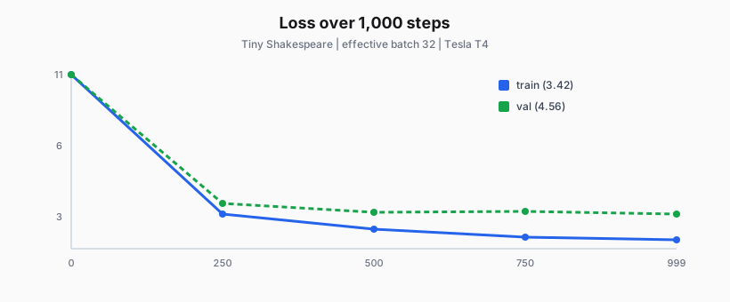
A few observations from staring at this:

1. The first jump is huge. Random init on a 50k vocab starts near "I have no idea." A few hundred steps later it already has a sense of the corpus.
2. Train keeps improving a bit after val flattens. On Tiny Shakespeare that is expected. The model is big relative to the data.
3. Best checkpoint landed at step 999 with val loss 4.56.

Total wall time was on the order of ten minutes of serious training on the T4, not counting the first eval.

And then I asked it to talk

Generation is just the forward pass in a loop.

@torch.no_grad()
def generate(self, idx, max_new_tokens, temperature=1.0, top_k=None):
    self.eval()
    for _ in range(max_new_tokens):
        idx_cond = idx[:, -self.config.block_size :]
        logits, _ = self(idx_cond)
        logits = logits[:, -1, :] / max(temperature, 1e-8)
        if top_k is not None:
            v, _ = torch.topk(logits, min(top_k, logits.size(-1)))
            logits[logits < v[:, [-1]]] = float("-inf")
        probs = F.softmax(logits, dim=-1)
        idx_next = torch.multinomial(probs, num_samples=1)
        idx = torch.cat([idx, idx_next], dim=1)
    self.train()
    return idx

Read it top to bottom:

1. Crop to the last block_size tokens. The model cannot see farther than that anyway.
2. Take only the last position's logits. That is the next-token distribution.
3. Divide by temperature. Lower = sharper / more confident. Higher = more random.
4. Optional top-k: zero out everything outside the top candidates before softmax.
5. Sample one token, append, repeat.

This is also where you first feel why the KV cache matters in real serving. Here I recompute attention over the whole prefix every step. That is fine for a toy. It is not fine at production scale.

Prompt:

prompt = "ROMEO:"
start = torch.tensor([enc.encode_ordinary(prompt)], dtype=torch.long, device=device)
out = model.generate(start, max_new_tokens=300, temperature=0.8, top_k=40)
print(enc.decode(out[0].tolist()))

Sample of what came out:

ROMEO:
And I am I tell thee for myself.

ROMEO:
I am not; I'll not so do to love me.

ROMEO:
What news, I'll bear my wife?

BENVOLIO:
'Tis not to my lie in love.

Nurse:
Well, sir, I will make me a word:
I do not a son, which I'll tell you
That I'll make for her to help me for her
And for my master.

FRIAR LAURENCE:
I would be so, I shall be not,
And in my life, and I'll give me; a word for,
As I shall I say she be here,
I do myself.

Is it good Shakespeare? No.

Does it know the shape of the dataset? Yes.

Speaker labels. Line breaks. Thee / I'll / Nay. Characters walking on stage who belong in the play. Syntax that is half-right and half-dream.

That is exactly what a short overfit-friendly run on Tiny Shakespeare should look like.

If the output had been random Unicode soup, the bug would be in the model. If the output had been perfect iambic pentameter after 1,000 steps on 300k tokens, I would not trust the experiment.

What this connected back to

Building the notebook made the earlier articles feel less separate.

• Causal masking is not optional. Without it, next-token training is label leakage.
• Multi-head attention is just several smaller attentions packed into one matmul.
• The KV story from the serving articles does not show up here yet, because I am training, not decoding at scale. But once you write generate(), you feel why people care about caching keys and values.
• Absolute learned positions (wpe) are simpler than RoPE. GPT-2 used them. Modern models often do not. Seeing both helps.

The point of training a small model is not to ship it.

The point is to close the loop between:

math on a page  →  modules in PyTorch  →  a loss curve  →  text that looks intentional

If you want to reproduce it

Rough outline of the notebook:

1. Download Tiny Shakespeare
2. Encode with tiktoken GPT-2 BPE
3. Build sliding-window (x, y) batches
4. Implement CausalSelfAttention → MLP → Block → GPT2
5. Train with AdamW, warmup, grad clip, grad accumulation
6. Sample from a prompt like ROMEO:

If you OOM:

• lower block_size
• lower BATCH_SIZE
• raise GRAD_ACCUM_STEPS so the effective batch stays sane

And if you want the full 124M GPT-2 Small shape, keep the same code and change the config. The architecture does not care. Your GPU does.

Takeaway

I did not train a foundation model.

I trained a recognizable GPT-2 stack on a tiny corpus until it learned the dialect of that corpus well enough to continue a Romeo line.

The code above is the whole machine in miniature: config, batches, attention, blocks, loss, sampling.

Once you have done this once, attention stops being a sequence of blog posts. It becomes a machine you can assemble, shrink to fit a T4, and listen to while it learns.